The Shapiro-Keyser (S–K) cyclone model was formulated in 1990 as a new conceptual model, developed in order to reconcile differences between observations of rapidly developing cyclones that diverged from that of the well-accepted Norwegian model.

S–K cyclogenesis is favoured by flat and confluent upper flow (Shapiro, Keyser, 1990 and McCallum, Norris, 1990), typically accompanied by acceleration normal to the flow found in the right jet entrance region.

Flat trough, confluent flow cyclogenesis results in an elongated hook-shaped region of cloud to the poleward side of the cyclone centre, known as the cloud head. (Young, 1995). This is associated with strong frontogentic development to the north of the system, and leads to the initial depression becoming stretched zonally. This stretching of the depression is accompanied by formation of a marked and thermally strong warm front (in some cases, as occurred in the ‘Great Storm of 1987’ a gradient of 8°C, over a distance of less than 20 km).

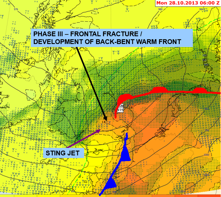
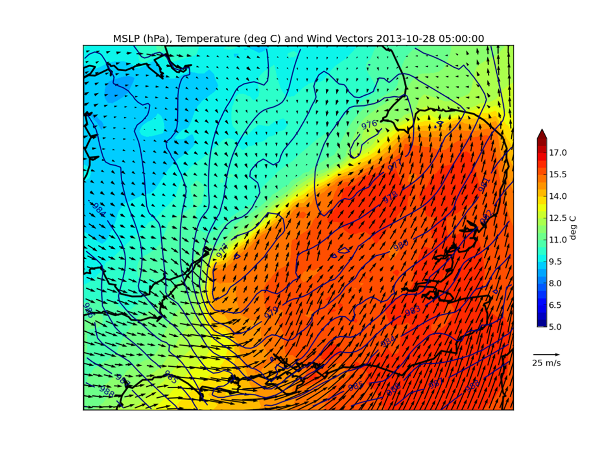
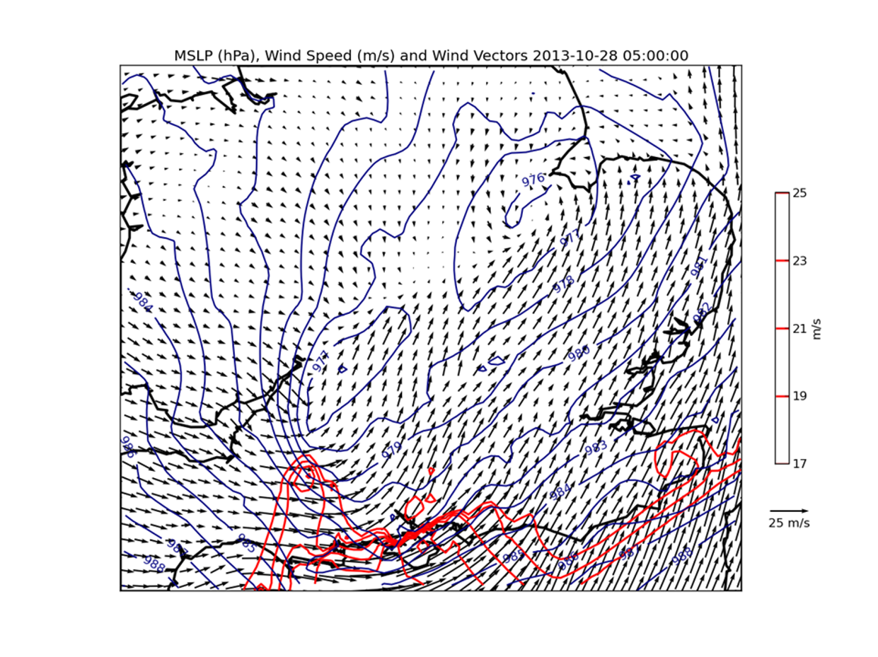
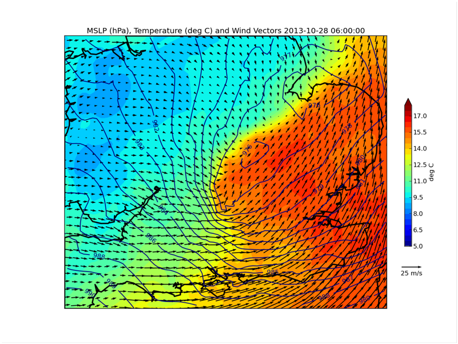
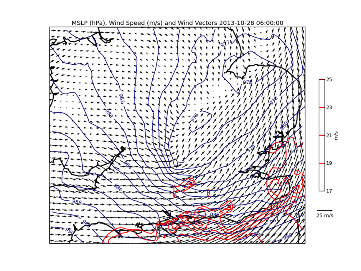
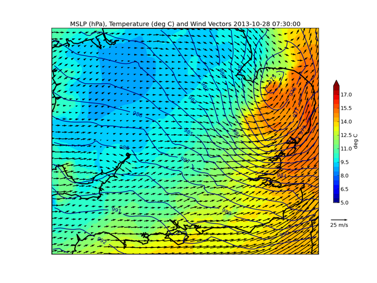
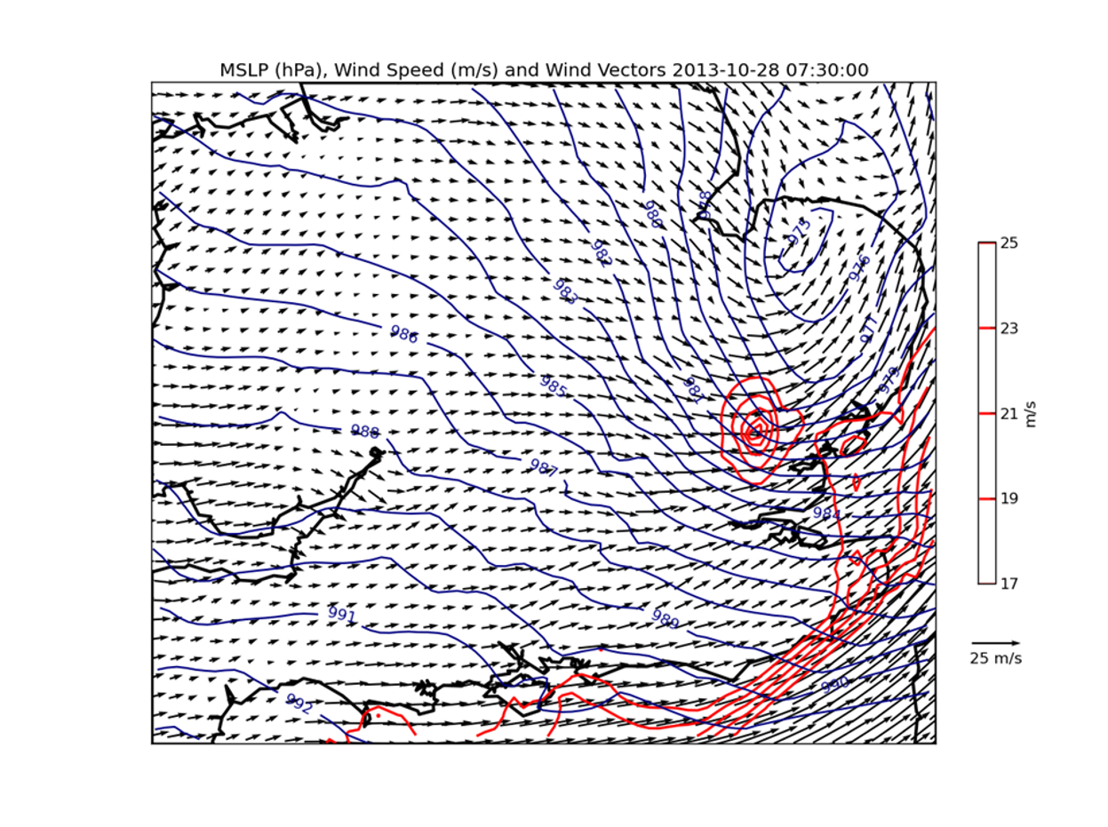
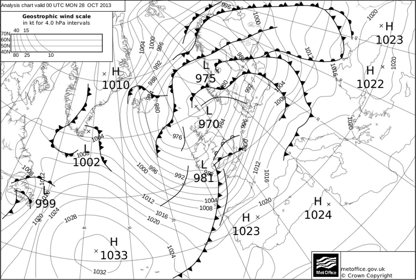
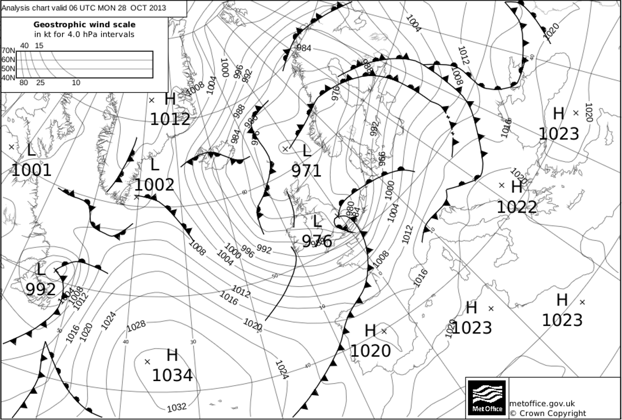
In the case of the St. Jude's Day Storm, many related circumstances that relate to S-K cyclogenesis were present. A more active and zonally stretched warm front with a very marked thermal gradient along it, and a weaker fragmented cold front which was separated from its associated warm front by a warm seclusion were both present - this can be seen in the 06 Z analysis, Figure 1, below) and my own analysis using NWP output (below right).

Sting Jets

Quasi-geostrophic (Q-G) theory on its own can explain the large pressure rises and associated intense pressure gradient that occur behind an explosively-deepening depression. Research shows that the sting jet development is a separate process that results in anomalously strong gusts at the surface.

Not all S–K cyclones develop a sting jet. However those that do tend to develop during the ‘frontal fracture’, forming to the south and southeast of the centre of the surface depression, this typically between the ‘bent–back’ warm front and the fractured cold front, before becoming replaced (undercut) by the CCB/CJ flow by stage III. They therefore do not last (in all cases) for more than a few hours.

The sting jet is a narrow corridor (~varying 20–200 km across) of very intense surface winds. SJ events can typically last between 1 and 12 hours (with the case studies of the ‘Great Storm of 1987’ and the ‘St Jude’ storm of 2013 observed to contain a long lasting sting jet), and lead to a localised period of damaging winds if the sting jet makes landfall.

The sting jet is theorised (Browning, 2004) to originate within the cloud head at a mid-tropospheric level of around 650-600 hPa, and back trajectory analysis (from Clark et al, 2005) supports this theory. From this level, the sting jet then descends to the top of the boundary layer, over a period of 3 to 4 hours. The descent accelerates on a level of constant өw (wet bulb potential temperature) from approximately 20 ms–1 at the cloud head, to over 45 ms−1; however this varies according to the intensity of the system.

Conditional symmetric instability (CSI) is thought to be crucial in the development of sting jets; numerical model simulations have shown circulations consistent with CSI and its presence has been inferred from satellite imagery by the presence of banded structures of a broadly similar scale. The body of evidence would therefore suggest that CSI plays an important role in the development of sting jets.

It is thought that cooling brought about by latent heat extraction from evaporating or melting of snow falling from the WCB into the descending air leads to a decrease in buoyancy within the SJ and therefore contributes to the downward acceleration.

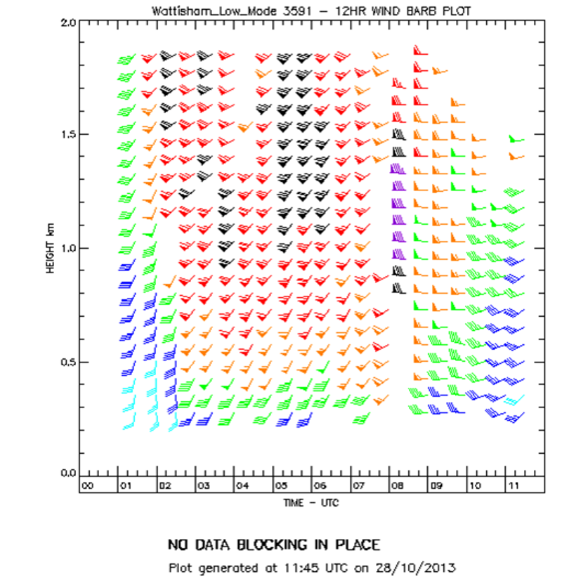
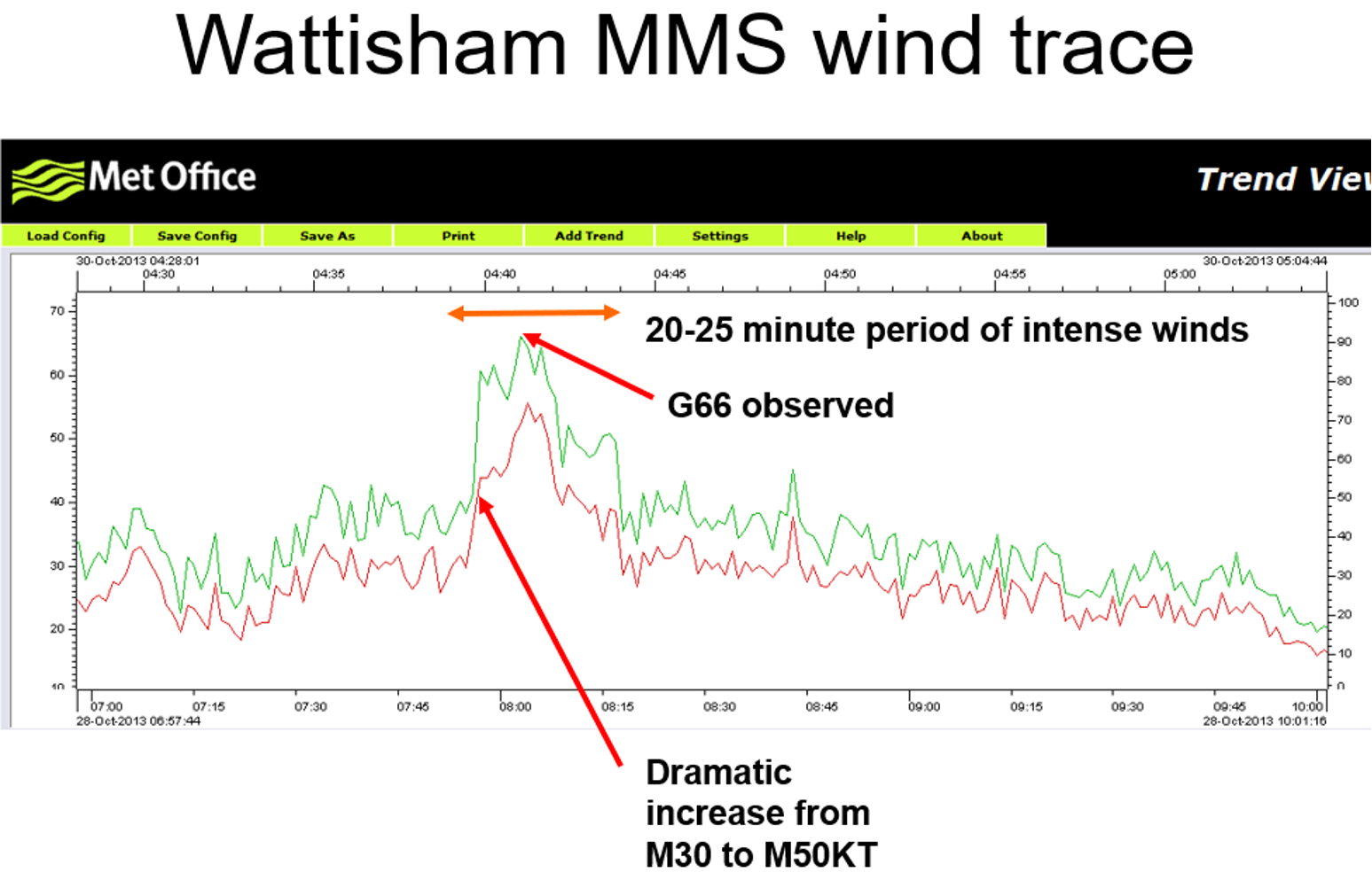
Below (Figure 2) is the wind trace taken from Wattisham where the winds increased suddenly at 0755 Z (0755 Local Time) from a mean of around 30 knots to 50 knots with gusts to 66 knots at its peak. This was a sudden and intense spell of very strong winds over a short period of time (20-25 minutes) and unfortunately occurred over a highly populated area of the UK at peak rush hour with many incidents due to the strong winds picking up suddenly.

References / Further Reading:

Development of a prototype real-time sting-jet precursor tool for forecasters

Browning K, 2004 The Sting at the end of the tail: Damaging winds associated with extratropical cyclones, Quarterly Journal of the Royal Meteorological Society, 130: 375-399.

Browning K, Smart D.J, Clark M.R., Illingworth A.J., 2015 The role of evaporating showers in the transfer of sting-jet momentum to the surface, Quarterly Journal of the Royal Meteorological Society, 141: 2956-2971.

Clark P.A., Browning K., Wang C., 2005 The string at the end of the tail: Model diagnostics of fine-scale three-dimensional structure of the cloud head, Quarterly Journal of the Royal Meteorological Society, 131: 2263–2292.

McCallum, E. and Norris, W.J.T., 1990: The storms of January and February 1990. Meteorology Mag, 119, 201-210.

Shapiro, M.A. and Keyser, D., 1990: Fronts, jet streams and the tropopause (In C. Newton and E. O. Holopainen, editors), Extratropical cyclones: the Eric Palm’en memorial volume (Chapter 10), American Meteorlogical Society, Boston, 167–191.

Young, M.V., 1995: Types of cyclogenesis, Images in Weather Forecasting (M.J. Bader, G.S. Forbes, J.R. Grant, R.B.E. Lilley, and A.J. Waters, Eds.) Cambridge University Press, 213–286.